Sample Size Calculation with G*Power
Sample size calculation is a critical step in experimental design.
If the sample size is too small, the study may be underpowered, increasing the risk of missing a true effect (Type II error).
If the sample size is too large, it can waste resources and, in clinical trials, unnecessarily expose participants to potential risks.
The goal of sample size calculation is to determine the smallest number of observations needed to reliably detect a meaningful effect while balancing statistical rigor, efficiency, and ethical considerations.
Let’s go step by step through the procedure using a two-sample, two-sided t-test for comparing means.
Setup
Let
\[ X_1,\dots,X_n \sim \mathcal{N}(\mu_1, \sigma^2), \qquad Y_1,\dots,Y_n \sim \mathcal{N}(\mu_2, \sigma^2), \]
independent, with equal group sizes \(n\).
We test
\[ H_0: \mu_1 - \mu_2 = 0 \qquad \text{vs.} \qquad H_1: \mu_1 - \mu_2 = \Delta, \]
where \(\Delta\) is the smallest difference we want to detect, at type I error \(\alpha\) and type II error \(\beta\) (statistical power \(1 - \beta\) ).
Let’s take a closer look to the Type I error and the Power.
Understand \(\alpha\) and \(\beta\)
The definition for “Type I Error” is “rejecting \(H_0\) when \(H_0\) is true”. We have
\[ \alpha \] \[ = P(\text{Reject } H_0 | H_0 \text{ is true.}) \] \[ = P(\text{Reject } H_0 | \mu_1 - \mu_2 = 0) \]
The definition for “Type II Error” is “failing to reject \(H_0\) when \(H_1\) is true”.
The difference of sample means has
\[ \bar{X} - \bar{Y} \sim \mathcal{N}\!\left( \mu_1 - \mu_2, \; \frac{2\sigma^2}{n} \right). \]
The corresponding z-statistic is
Under \(H_0\), we have \(\mu_1 - \mu_2 = 0\) and \(\bar{X} - \bar{Y} \sim N(0, \frac{2\sigma^2}{n})\) , Thus
\[ Z=\frac{(\bar{X} - \bar{Y)}}{\sqrt{2\sigma^2/n}} \sim N(0,1) \]
Under \(H_1\), we have \(\mu_1 - \mu_2 = \Delta\), and \(\bar{X} - \bar{Y} \sim N(\Delta, \frac{2\sigma^2}{n})\) , Thus
\[ \frac{\bar{X}-\bar{Y}}{\sqrt{2\sigma^2/n}} \sim N(\frac{\Delta}{\sqrt{2\sigma^2/n}}, 1) = N(\delta, 1) \]
Rejection Region
If the null hypothesis is true, the difference between \(\bar{X}\) and \(\bar{Y}\) should be close to 0. When the observed difference \(\bar{X}-\bar{Y}\) is unusually large or small, for example, \(\bar{X}-\bar{Y}=5\) or \(\bar{X}-\bar{Y}=-10\) , the data provide evidence against \(H_0\) and support the alternative hypothesis \(H_1\) , suggesting that the true means of \(X\) and \(Y\) are not equal.
This idea can be expressed in standardized form:
if the null is true, the test statistic \(Z\) follows a standard normal distribution, \(Z \sim N(0,1)\) . We reject \(H_0\) when the observed \(Z_\text{observed}\) is either too high or too low. That is, when the absolute value \(|Z_\text{observed}|\) is large. But how large is “large enough”? The p-value answers that question.
The p-value represents the probability, under the null hypothesis, of observing a result as extreme or more extreme than what we obtained. For example, if \(Z_\text{observed}=2\) , the corresponding tail probability is \(P(|Z| \geq 2)\) where \(Z \sim N(0,1)\) under \(H_0\) . A larger \(|Z_\text{observed}|\) leads to a smaller p-value. Therefore, the rule “reject the null when p-value < \(\alpha\)” is equivalent to “reject the null if \(|Z_\text{observed}| > z_{1-\alpha/2}\) .” For example, if \(\alpha=0.05\), we reject the null if \(|Z_\text{observed}|\geq z_{0.975}=1.96\) .
For a given \(\alpha\), the rejection region is:
\[ |Z_\text{observed}| > z_{1 - \alpha/2} \]
Statistical Power
The statistical power is define as \(1-\beta\) where \(\beta\) is the probability of making type II error. Using the results
\[ 1-P(A|B) = P(A^C|B) \]
where “\(A^C\)” is the complement of \(A\). We have
\[ 1-\beta \] \[ = P(\text{Reject } H_0 | H_1 \text{ is true}) \] \[ =P(\text{Reject } H_0 | \mu_1 - \mu_2 = \Delta). \]
Now using the results from the previous section,
\[ \text{Reject } H_0 = |Z_\text{observed}| \geq z_{1-\alpha/2} \]
\[ H_1 \text{ is true } = \frac{\bar{X}-\bar{Y}}{\sqrt{2\sigma^2/n}} \sim N(\delta, 1) \]
Then the power is
\[ 1 - \beta = P(|Z_\text{observed}| > z_{1-\alpha/2} ) \text{ when } Z_\text{observed} \sim \mathcal{N}(\delta, 1)) \quad . \]
Now let’s rewrite this probability in a standard normal distribution
\[ P(|Z_\text{observed}|>z_{1-\alpha/2}) \] \[ = P(|Z_\text{observed} -\delta|> z_{1-\alpha/2} - \delta) \] \[ =P(Z \geq z_{1-\alpha/2}-\delta) + P(Z\leq -z_{1-\alpha/2} - \delta) \]
To maintain a high statistical power (say this probability should higher than 0.9), we will need to have
\[ \delta \geq z_{1-\alpha/2} + z_{1-\beta} \] Thus, the required per-group sample size is:
\[ \boxed{ n \geq \frac{2\sigma^2}{\Delta^2} \big( z_{1-\alpha/2} + z_{1-\beta} \big)^2 } \]
and the total sample size (two groups) is \(N = 2n\).
What is G*Power?
G*Power is a free software tool (Windows/Mac) that allows researchers to compute required sample sizes, achieved power, or effect sizes for a wide variety of statistical tests (t-test, ANOVA, regression, correlations, etc). It is commonly used in psychology, medicine, and social sciences. It’s user-friendly, with point-and-click menus (no coding needed).
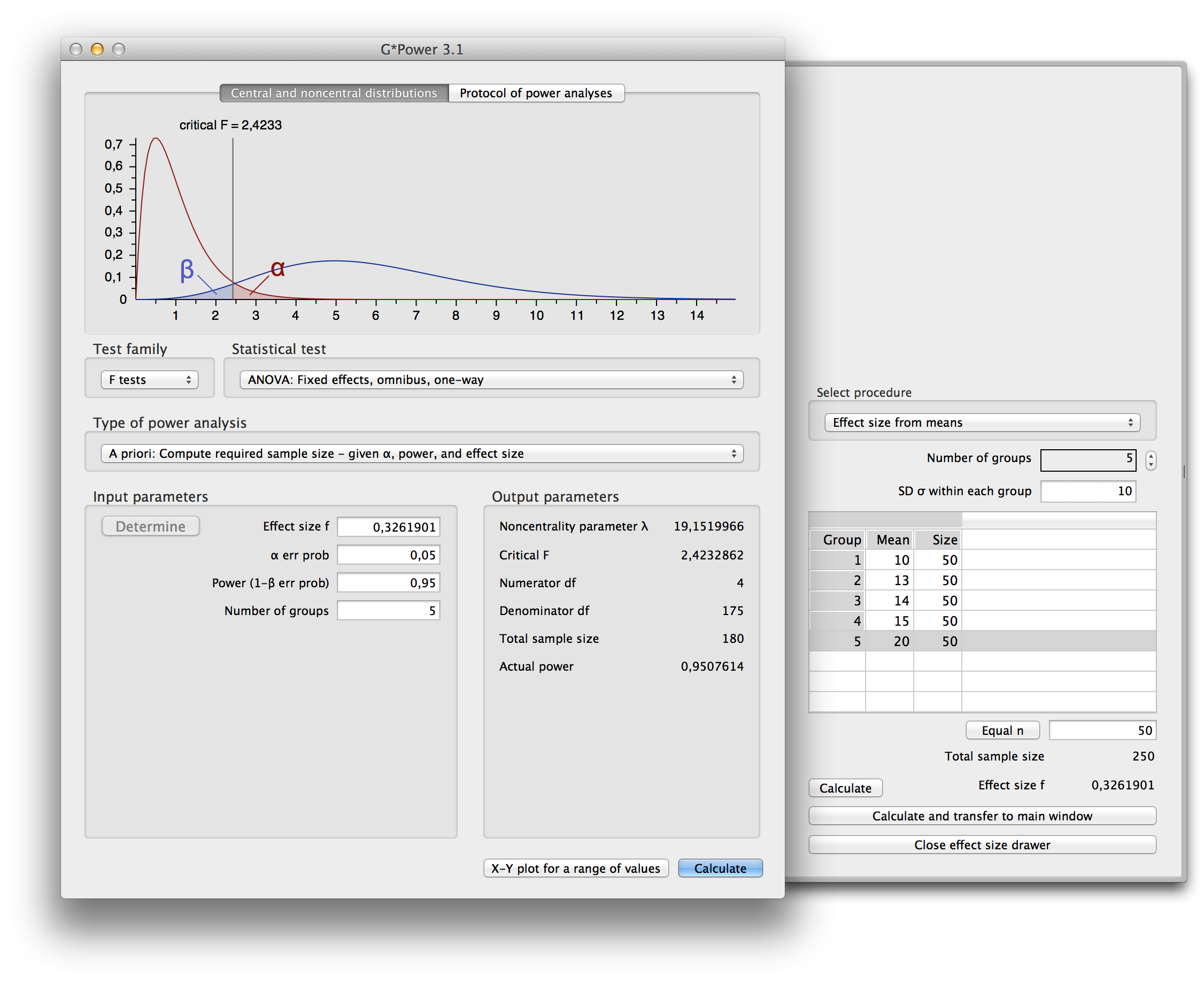
G*Power conducts the following types of analysis:
A priori: Find n given α, power, and effect size.
Post hoc: Find power given n.
Sensitivity: Find smallest effect detectable.
Compromise: Balance α and β.