Code
# install.packages(c("strucchange", "changepoint", "ocp"))
library("strucchange")
library("changepoint")
library("ocp")
library("knitr")# install.packages(c("strucchange", "changepoint", "ocp"))
library("strucchange")
library("changepoint")
library("ocp")
library("knitr")changepoint)Now let’s detect changes in mean and variance.
set.seed(42)
y <- c(rnorm(50, 10, 1), rnorm(50, 15, 1), rnorm(50, 12, 1))
plot(y, type = "l", main = "Simulated Data with Mean Shifts", xlab = "Time", ylab = "Value")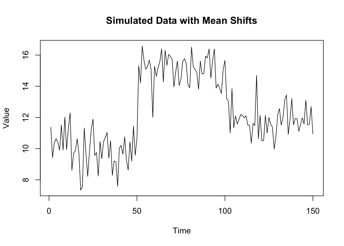
The goal is to detect where the mean of a sequence suddenly changes, for example, when a process shifts from one stable level to another.
We assume a simple model:
\[ y_t \sim N(\mu_i, \sigma^2) \]
where each segment \(i\) has its own mean \(\mu_i\). There are unknown changepoints where the mean of the distribution shifted. The algorithm will find the number and the locations of those changepoints.
The algorithm cut the data into segments where each piece has a constant mean, and find where those cuts make the data fit best.
For each possible segmentation, minimize the sum of squared deviation from the segment mean (similar to decision tree) \[ \sum(y_t - \hat{\mu})^2 \]
Add a penalty (e.g. BIC, AIC) on the number of breaks to avoid too many change points(similar to pruning a tree).
cpt_mean <- cpt.mean(y, method = "PELT")
plot(cpt_mean, main = "Detected Change Points (Mean)")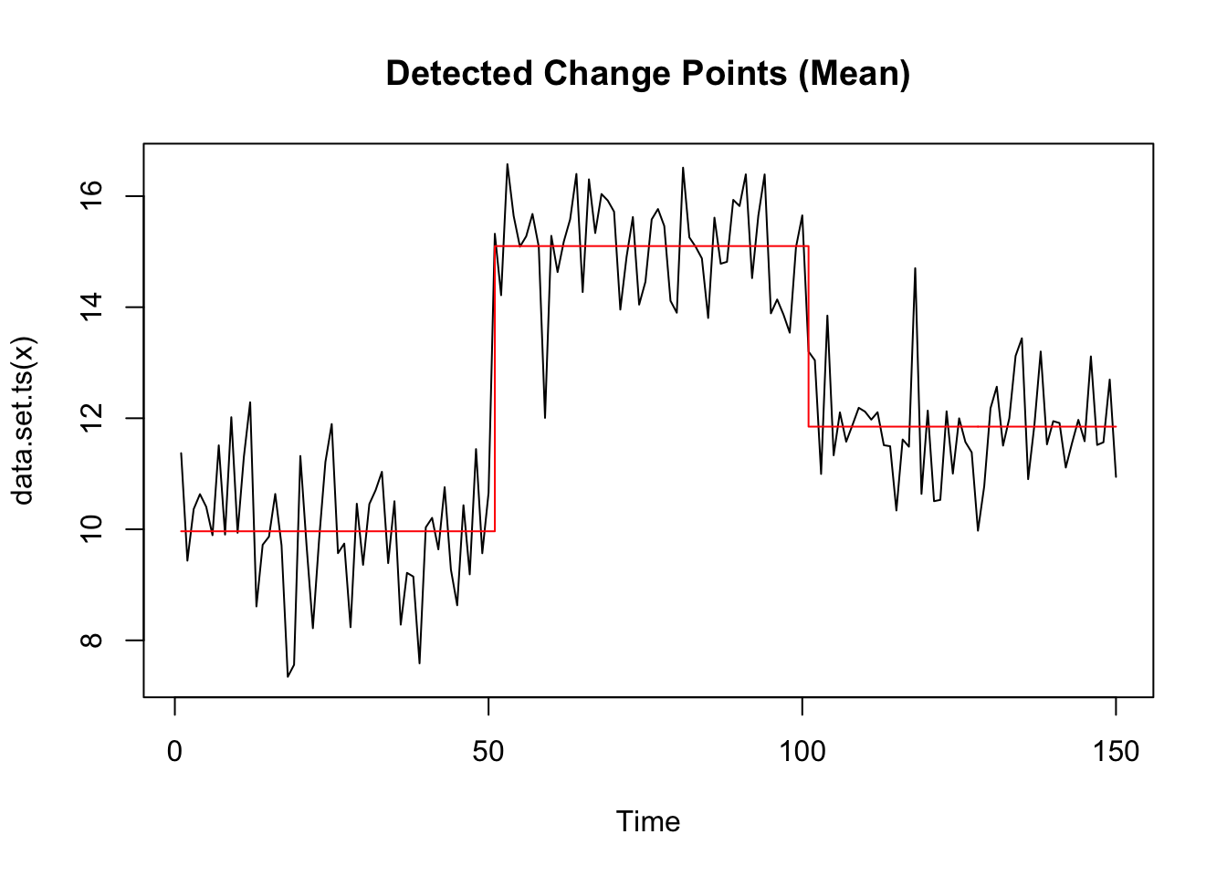
cpt.mean() only detects the mean changes across segments. cpt.meanvar() allows both the mean and the variance to shift. We asusme
\[ y_t \sim N(\mu_i, \sigma_i^2) \]
where both \(\mu_i\) and \(\sigma_i^2\) may change. This is especially useful when the signal’s level and volatility both change. For example, in financial returns, climate data, or sensor measurements.
Conceptually, cpt.meanvar() is the same as cpt.mean() and minimize a “cost+penalty” function but with a new cost on the variance. The rest of the algorithm is identical.
cpt_meanvar <- cpt.meanvar(y, method = "PELT")
plot(cpt_meanvar, main = "Detected Change Points (Mean & Variance)")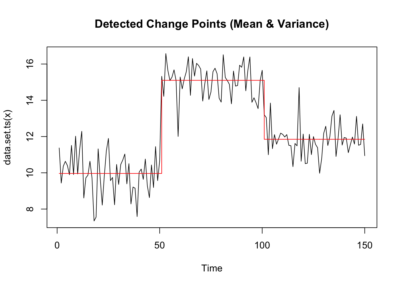
method defines the search strategy
| Method | Meaning | Description |
|---|---|---|
AMOC |
At Most One Change | Finds a single change point only — the simplest case. |
BinSeg |
Binary Segmentation | Repeatedly splits the data where the biggest change occurs, then applies the same search within each segment. It’s a fast, approximate method. |
SegNeigh |
Segment Neighborhood | Searches all combinations of breakpoints up to a maximum number. It’s exact but slow for large data. |
PELT |
Pruned Exact Linear Time | Uses dynamic programming and pruning rules to find the exact global optimum very efficiently. It’s usually the best choice for large datasets. |
Typical choice: PELT
penalty: How it balances fit vs. simplicity
| Penalty | Meaning | Description |
|---|---|---|
| `AIC` | Akaike Information Criterion | Allows more change points |
| `BIC` | Bayesian Information Criterion | More penalty on changes. More conservative, fewer changes |
| `MBIC` | Modified BIC | Adds stronger penalty for small samples. Often the default . |
| `Mannual` | User-specified | Full control |
Typical choice: MBIC
cpt.mean(y, method = "AMOC")Class 'cpt' : Changepoint Object
~~ : S4 class containing 12 slots with names
cpttype date version data.set method test.stat pen.type pen.value minseglen cpts ncpts.max param.est
Created on : Thu Oct 23 09:56:53 2025
summary(.) :
----------
Created Using changepoint version 2.3
Changepoint type : Change in mean
Method of analysis : AMOC
Test Statistic : Normal
Type of penalty : MBIC with value, 15.03191
Minimum Segment Length : 1
Maximum no. of cpts : 1
Changepoint Locations : 50 cpt.mean(y, method = "BinSeg")Class 'cpt' : Changepoint Object
~~ : S4 class containing 14 slots with names
cpts.full pen.value.full data.set cpttype method test.stat pen.type pen.value minseglen cpts ncpts.max param.est date version
Created on : Thu Oct 23 09:56:53 2025
summary(.) :
----------
Created Using changepoint version 2.3
Changepoint type : Change in mean
Method of analysis : BinSeg
Test Statistic : Normal
Type of penalty : MBIC with value, 15.03191
Minimum Segment Length : 1
Maximum no. of cpts : 5
Changepoint Locations : 50 100
Range of segmentations:
[,1] [,2] [,3] [,4] [,5]
[1,] 50 NA NA NA NA
[2,] 50 100 NA NA NA
[3,] 50 100 12 NA NA
[4,] 50 100 12 102 NA
[5,] 50 100 12 102 11
For penalty values: 407.2563 261.161 7.669837 2.729663 2.644968 strucchange)We begin with the structural change model, a regression that allows for multiple linear segments. The idea is simple: your data might not follow one single regression line. At some unknown points, the relationship between \(x\) and \(y\) may change, for example, after a policy shift, new technology, or climate event. breakpoints() looks for those points, called structural breaks, by splitting the data into several straight-line segments and finding where the fit improves the most.
It does this by:
Fitting linear models for all possible ways of dividing the data into pieces. Usually from 0 breakpoint to a pre-selected maximum number of breaks.
Choosing the split points that minimize the overall sum of squared residuals(RSS) for each given number of breakpoints.
Selecting how many breaks to keep using a BIC score to balance fit and simplicity.
Load a simple real dataset:
## Nile data with one breakpoint: the annual flows drop in 1898
## because the first Ashwan dam was built
data("Nile")
plot(Nile, main = "Annual Flow of the Nile River", ylab = "Flow", xlab = "Year")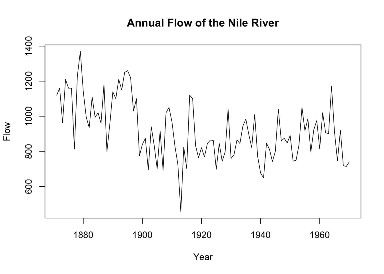
## F statistics indicate one breakpoint
fs.nile <- Fstats(Nile ~ 1)
plot(fs.nile)
breakpoints(fs.nile)
     Optimal 2-segment partition:

Call:
breakpoints.Fstats(obj = fs.nile)

Breakpoints at observation number:
28

Corresponding to breakdates:
1898 lines(breakpoints(fs.nile))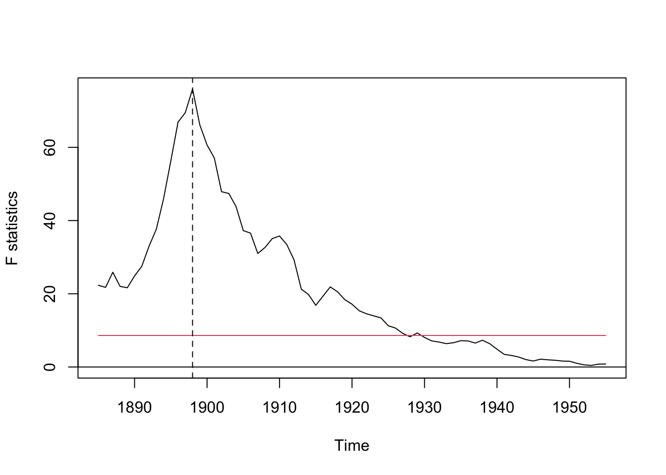
## or
bp.nile <- breakpoints(Nile ~ 1)
summary(bp.nile)
     Optimal (m+1)-segment partition:

Call:
breakpoints.formula(formula = Nile ~ 1)

Breakpoints at observation number:

m = 1      28
m = 2      28       83
m = 3      28    68 83
m = 4      28 45 68 83
m = 5   15 30 45 68 83

Corresponding to breakdates:

m = 1        1898
m = 2        1898           1953
m = 3        1898      1938 1953
m = 4        1898 1915 1938 1953
m = 5   1885 1900 1915 1938 1953

Fit:

m   0       1       2       3       4       5
RSS 2835157 1597457 1552924 1538097 1507888 1659994
BIC 1318 1270 1276 1285 1292 1311## the BIC also chooses one breakpoint
plot(bp.nile)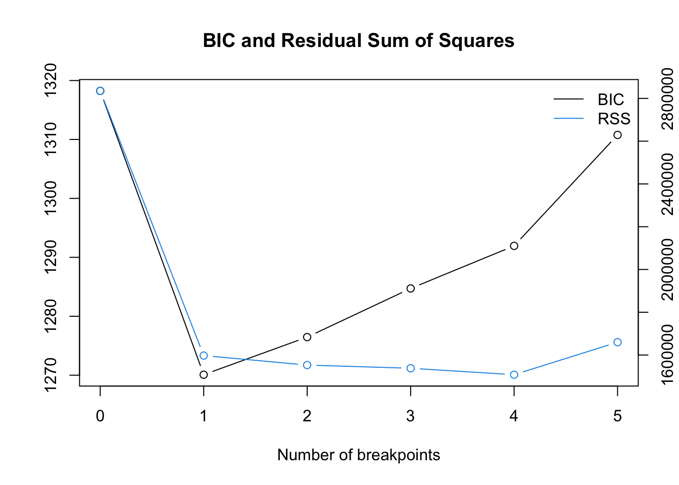
breakpoints(bp.nile)
     Optimal 2-segment partition:

Call:
breakpoints.breakpointsfull(obj = bp.nile)

Breakpoints at observation number:
28

Corresponding to breakdates:
1898 ## fit null hypothesis model and model with 1 breakpoint
fm0 <- lm(Nile ~ 1)
fm1 <- lm(Nile ~ breakfactor(bp.nile, breaks = 1))
plot(Nile)
lines(ts(fitted(fm0), start = 1871), col = 3)
lines(ts(fitted(fm1), start = 1871), col = 4)
lines(bp.nile)
## confidence interval
ci.nile <- confint(bp.nile)
ci.nile
     Confidence intervals for breakpoints
     of optimal 2-segment partition:

Call:
confint.breakpointsfull(object = bp.nile)

Breakpoints at observation number:
  2.5 % breakpoints 97.5 %
1    25          28     32

Corresponding to breakdates:
  2.5 % breakpoints 97.5 %
1 1895 1898 1902lines(ci.nile)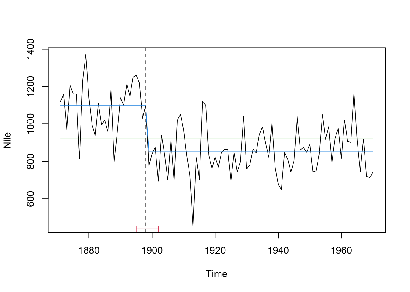
A more advanced example:
## UK Seatbelt data: a SARIMA(1,0,0)(1,0,0)_12 model
## (fitted by OLS) is used and reveals (at least) two
## breakpoints - one in 1973 associated with the oil crisis and
## one in 1983 due to the introduction of compulsory
## wearing of seatbelts in the UK.
data("UKDriverDeaths")
seatbelt <- log10(UKDriverDeaths)
seatbelt <- cbind(seatbelt, lag(seatbelt, k = -1), lag(seatbelt, k = -12))
colnames(seatbelt) <- c("y", "ylag1", "ylag12")
seatbelt <- window(seatbelt, start = c(1970, 1), end = c(1984,12))
plot(seatbelt[,"y"], ylab = expression(log[10](casualties)))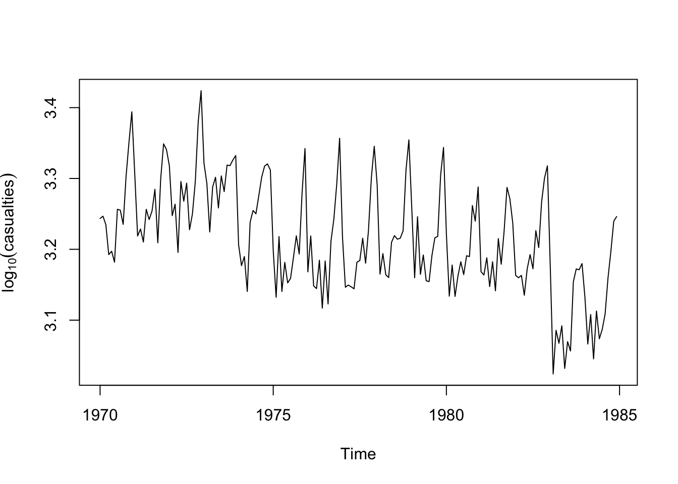
## testing
re.seat <- efp(y ~ ylag1 + ylag12, data = seatbelt, type = "RE")
plot(re.seat)

## dating
bp.seat <- breakpoints(y ~ ylag1 + ylag12, data = seatbelt, h = 0.1) # h: minimum proportion of the data in each segment
summary(bp.seat)
     Optimal (m+1)-segment partition:

Call:
breakpoints.formula(formula = y ~ ylag1 + ylag12, h = 0.1, data = seatbelt)

Breakpoints at observation number:

m = 1      46
m = 2      46                   157
m = 3      46 70                157
m = 4      46 70    108         157
m = 5      46 70        120 141 160
m = 6      46 70 89 108     141 160
m = 7      46 70 89 107 125 144 162
m = 8   18 46 70 89 107 125 144 162

Corresponding to breakdates:

m = 1           1973(10)
m = 2           1973(10)                                             1983(1)
m = 3           1973(10) 1975(10)                                    1983(1)
m = 4           1973(10) 1975(10)         1978(12)                   1983(1)
m = 5           1973(10) 1975(10)                  1979(12) 1981(9)  1983(4)
m = 6           1973(10) 1975(10) 1977(5) 1978(12)          1981(9)  1983(4)
m = 7           1973(10) 1975(10) 1977(5) 1978(11) 1980(5)  1981(12) 1983(6)
m = 8   1971(6) 1973(10) 1975(10) 1977(5) 1978(11) 1980(5)  1981(12) 1983(6)

Fit:

m   0         1         2         3         4         5         6
RSS    0.3297    0.2967    0.2676    0.2438    0.2395    0.2317    0.2258
BIC -602.8611 -601.0539 -598.9042 -594.8774 -577.2905 -562.4880 -546.3632

m   7         8
RSS    0.2244    0.2231
BIC -526.7295 -506.9886lines(bp.seat, breaks = 2)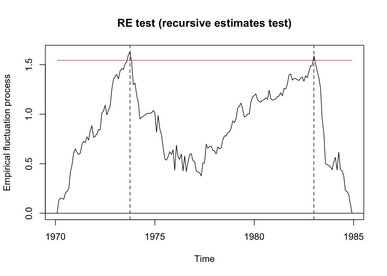
## minimum BIC partition
plot(bp.seat)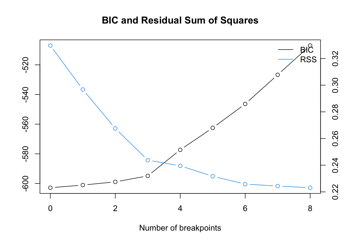
breakpoints(bp.seat)
     Optimal 1-segment partition:

Call:
breakpoints.breakpointsfull(obj = bp.seat)

Breakpoints at observation number:
NA

Corresponding to breakdates:
NA ## the BIC would choose 0 breakpoints although the RE and supF test
## clearly reject the hypothesis of structural stability. Bai &
## Perron (2003) report that the BIC has problems in dynamic regressions.
## due to the shape of the RE process of the F statistics choose two
## breakpoints and fit corresponding models
bp.seat2 <- breakpoints(bp.seat, breaks = 2)
fm0 <- lm(y ~ ylag1 + ylag12, data = seatbelt)
fm1 <- lm(y ~ breakfactor(bp.seat2)/(ylag1 + ylag12) - 1, data = seatbelt)
## plot
plot(seatbelt[,"y"], ylab = expression(log[10](casualties)))
time.seat <- as.vector(time(seatbelt))
lines(time.seat, fitted(fm0), col = 3)
lines(time.seat, fitted(fm1), col = 4)
lines(bp.seat2)
## confidence intervals
ci.seat2 <- confint(bp.seat, breaks = 2)
ci.seat2
     Confidence intervals for breakpoints
     of optimal 3-segment partition:

Call:
confint.breakpointsfull(object = bp.seat, breaks = 2)

Breakpoints at observation number:
  2.5 % breakpoints 97.5 %
1    33          46     56
2   144         157    171

Corresponding to breakdates:
  2.5 %    breakpoints 97.5 %
1 1972(9)  1973(10)    1974(8)
2 1981(12) 1983(1) 1984(3)lines(ci.seat2)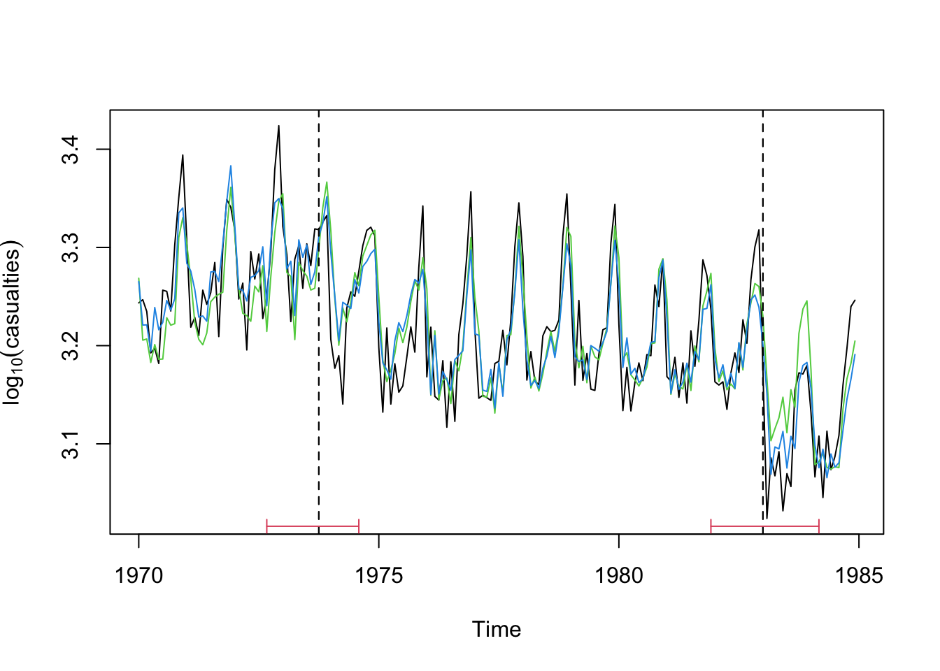
ocp)Most change point methods — like breakpoints() or cpt.mean() — work retrospectively: they look at all data at once and find where shifts happened. But in many real settings (finance, sensors, streaming data), you want to detect changes as data arrives. That’s where online Bayesian change point detection comes in. For this lab, we’ll focus only on running the code. The theoretical background will be covered next week.
The ocp package implements online Bayesian change point detection (Adams & MacKay, 2007). It infers posterior probabilities of a change in real time. At each new observation \(y_t\), we want to update our belief about whether a change has occurred. We define the run length \(r_t\) as the number of data points since the last change point.
The result is a probability of change at every new data point.
set.seed(123)
y3 <- c(rnorm(50, 5, 1), rnorm(50, 10, 1), rnorm(50, 7, 1))
plot(y3, type = 'l')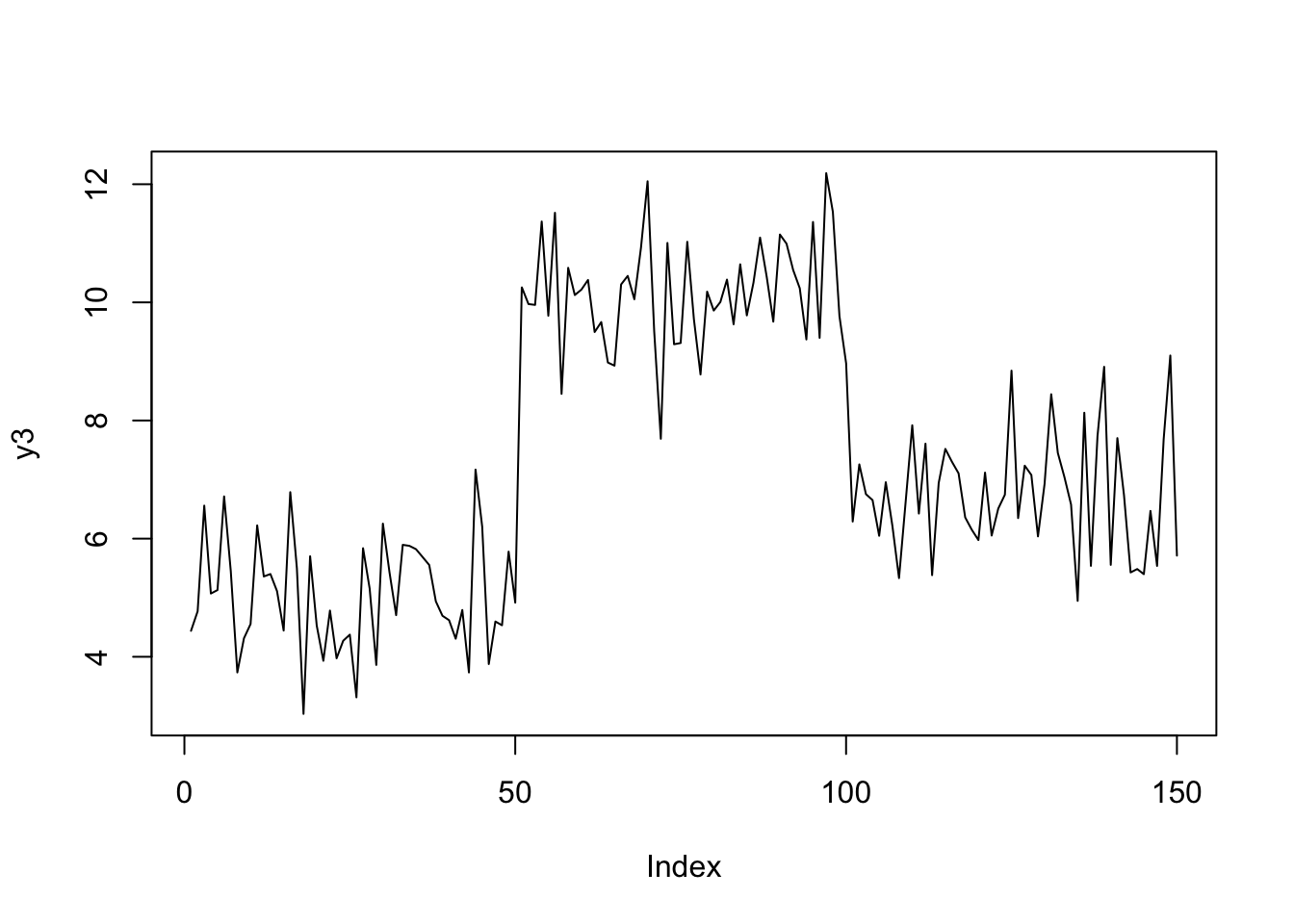
# running the basic function with all the default settings
ocp_result <- onlineCPD(y3, getR=TRUE)
summary(ocp_result)
[1] " An oCPD object:"
[1] "R vectors not truncated."
[1] "1 -variate data."
[1] "Attributes returned:"
[1] "R" "prevR" "prevRprod"
[4] "prevRsum" "prevDataPt" "time"
[7] "ocpd_settings" "threshcps" "max"
[10] "update_paramsT" "update_params0" "init_params"
[13] "logprobmaxes" "logprobcps" "currmu"
[16] "changepoint_lists"
[1] "Changepoints:"
[[1]]
[1] 1 51 101plot(ocp_result, main = "Online Bayesian Change Point Detection")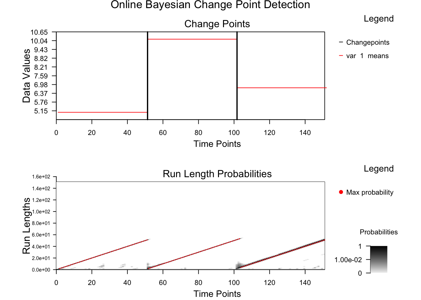
| Method | Type | Focus | Output | Strengths | Weaknesses |
|---|---|---|---|---|---|
strucchange |
Regression-based | Structural breaks in coefficients | Breakpoints, fitted model | Parametric interpretability | Linear assumption |
changepoint |
Frequentist | Mean/variance shifts | Detected indices | Fast, scalable | No uncertainty quantification |
ocp |
Bayesian (online) | Sequential change probabilities | Posterior probabilities | Works on streaming data, quantifies uncertainty | More complex output |
library(readr)
url <- "https://datahub.io/core/global-temp/r/monthly.csv"
temp <- read_csv(url)
plot(temp$Mean, type="l", main="Global Temperature Anomalies")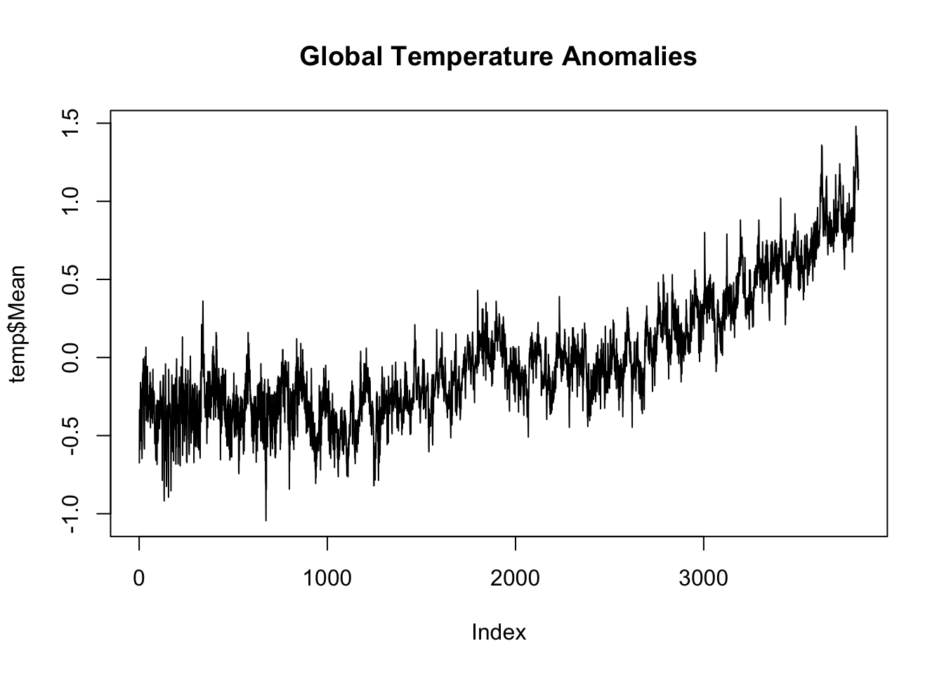
Apply all three change point detection methods to the global temperature dataset.
Perform any necessary data preparation, such as cleaning, smoothing, or time series decomposition.
Visualize and compare the detected change points from all three methods.