Swinging Door Algorithm and Bayesian Change Point Detection

Swinging Door Algorithm

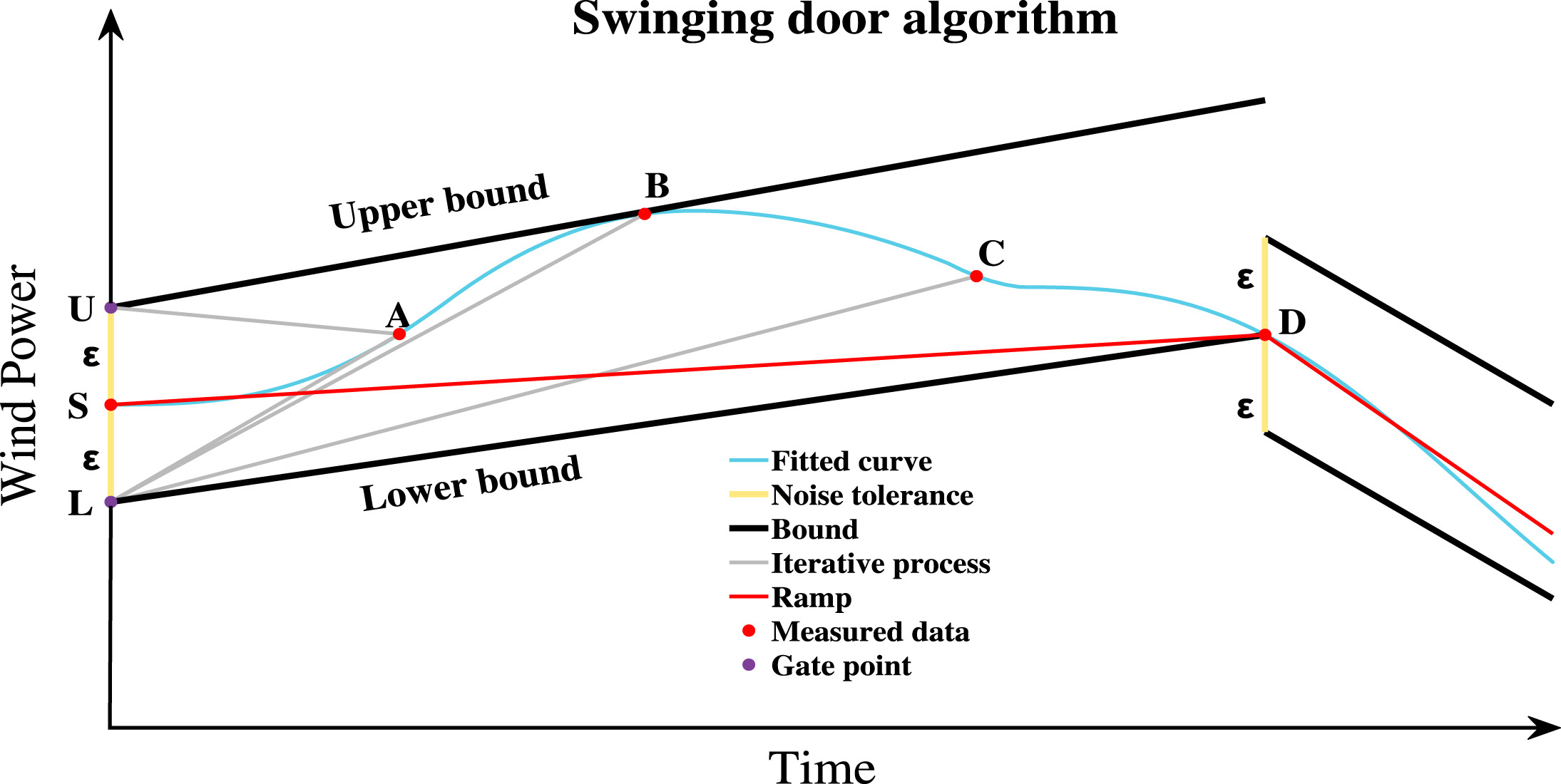
The Swinging Door Algorithm is a lossy down-sampling and compression algorithm for time-series or sequential data. It is designed for streaming or continuous monitoring data where huge numbers of data points are generated, but you don’t want to store every point if many of them lie along a nearly straight trend.

In essence, it monitors whether incoming data continue to lie within a “tolerance corridor” around an implied trend line;

• if they do, you skip storing them and keep the door open;

• if they diverge enough, you “close the door” (record the last point) and start a new segment.

The Core Logit

Suppose you have a sequence of observations

\[ \{ (t_1, x_1), (t_2, x_2), ..., (t_T, x_T)\} \] and a pre-defined tolerance parameter \(\epsilon>0\). At any point, Swinging Door Algorithm maintains:

• A start point \((t_s, x_s)\) for the current segment;
• Upper and lower slope bounds that describe how steep the line through \((t_s, x_s)\) can be while staying within the tolerance band(door).

For the first two observations \((t_1, x_1), (t_2, x_2)\), compute two initial slopes:

\[ m_{\text{u}} = \frac{(x_2+\epsilon)-x_1}{t_2-t_1}, m_{\text{l}} = \frac{(x_2-\epsilon)-x_1}{t_2-t_1} \] For new observation \((t_3, x_3)\), recalculate the slopes

\[ m_{\text{u,new}} = \frac{(x_3+\epsilon)-x_1}{t_3-t_1} \]

\[ m_{\text{l, new}} = \frac{(x_3-\epsilon)-x_1}{t_3-t_1} \]

Then update the running slope limit

\[ m_{u} = \text{min}(m_{u}, m_{\text{u,new}}) \]

\[ m_{l} = \text{max}(m_{l}, m_{\text{l,new}}) \]

If the two bounds cross (i.e. \(m_{l}>m_{u}\)), it means no single line can keep all point within \(\pm \epsilon\) band, the door breaks and a new segment starts. Then we only keep the first and the last observations in a segment and omit the others.

As long as \(m_l<m_u\) , we can find line with a a slope \(m\) such that \(m_l<m<m_u\) for every included point, so the whole segment sit inside the \(\pm \epsilon\) band around that line.

Check on the Shiny App on Swinging Door Algorithm.

How would you choose the \(\epsilon\) value in practice?

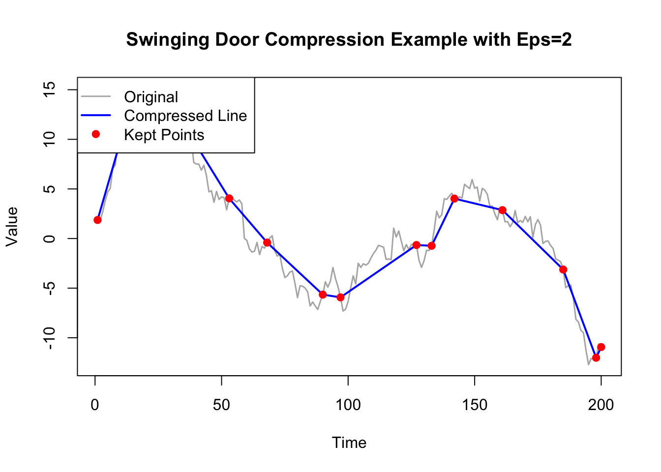
• A small \(\epsilon\) value makes a very sensitive door and many short segments.

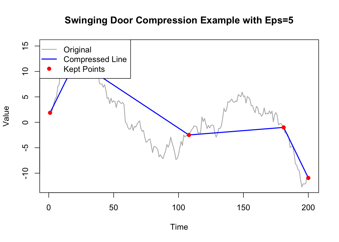
• A large \(\epsilon\) value makes the algorithm less sensitive, and fewer longer segments.

# --- Example: Swinging Door Algorithm with Plot ----

# Sample noisy time series
set.seed(42)
time <- 1:200
value <- cumsum(rnorm(200, 0, 1)) + 10 * sin(time / 20)

# --- Simple Swinging Door function ---
swinging_door <- function(time, value, eps = 2) {
  n <- length(time)
  keep <- c(1)
  anchor <- 1
  upper <- Inf
  lower <- -Inf
  
  for (i in 2:n) {
    dt <- time[i] - time[anchor]
    upper_i <- (value[i] + eps - value[anchor]) / dt
    lower_i <- (value[i] - eps - value[anchor]) / dt
    
    upper <- min(upper, upper_i)
    lower <- max(lower, lower_i)
    
    if (lower > upper) {
      keep <- c(keep, i - 1)
      anchor <- i - 1
      upper <- Inf
      lower <- -Inf
    }
  }
  keep <- c(keep, n)
  keep
}

# Apply algorithm
idx2 <- swinging_door(time, value, eps = 2)
compressed2 <- data.frame(time = time[idx2], value = value[idx2])

# --- Visualization ---
plot(time, value, type = "l", col = "grey70", lwd = 1.5,
     main = "Swinging Door Compression Example with Eps=2",
     xlab = "Time", ylab = "Value")
lines(compressed2$time, compressed2$value, col = "blue", lwd = 2)
points(compressed2$time, compressed2$value, col = "red", pch = 19)
legend("topleft", legend = c("Original", "Compressed Line", "Kept Points"),
       col = c("grey70", "blue", "red"), lwd = c(1.5, 2, NA), pch = c(NA, NA, 19))

# Apply algorithm
idx5 <- swinging_door(time, value, eps = 5)
compressed5 <- data.frame(time = time[idx5], value = value[idx5])

# --- Visualization ---
plot(time, value, type = "l", col = "grey70", lwd = 1.5,
     main = "Swinging Door Compression Example with Eps=5",
     xlab = "Time", ylab = "Value")
lines(compressed5$time, compressed5$value, col = "blue", lwd = 2)
points(compressed5$time, compressed5$value, col = "red", pch = 19)
legend("topleft", legend = c("Original", "Compressed Line", "Kept Points"),
       col = c("grey70", "blue", "red"), lwd = c(1.5, 2, NA), pch = c(NA, NA, 19))

How to choose \(\epsilon\)?

Usually we choose the \(\epsilon\) by

• business/physics tolerance (e.g. max absolute deviation you’re willing to ignore),

• or by sensor noise (e.g. estimated standard deviation \(\sigma\), then \(\epsilon \approx 3\sigma\) ). For data compression purpose,

• You can also choose \(\epsilon\) by the compression target (e.g. keep only 20% of the points).

• If you have labeled historical data, choose \(\epsilon\) by cross validation.

Online Bayesian Change Point Detection

The Swinging Door Algorithm (and all other methods we had so far) are purely deterministic, not probabilistic. The Bayesian version replaces the hard threshold \(\epsilon\) with probabilistic reasoning. At each new observation, we ask:

Given what we’ve seen, what is the probability that a change just occurred?

You test a sensor that sometimes gives false alarms. After seeing 3 alarms in a row, do you believe the system has truly failed, or was it just bad luck?

A Frequentist may say, let’s assume the system is fine, compute how unlikely 3 alarms in a row would be, and see if that’s small enough to reject that assumption. (p-value)

A Bayesian statistician may say, let’s combine what I already believe about the system (my prior) with the new evidence (the data) to update my belief.(adaptive learning)

So Bayesian methods are about belief updating. In the Bayesian view, probability measures how strongly we believe in a statement, given what we know. These beliefs can change as we gather more data.

You may have Bayes’ Theorem in DA220

\[ P(A|B) = \frac{P(B|A)P(A)}{P(B)} \]

Let’s look at two specific event “A” and “B”:

• “A”: a parameter \(\theta\), or a hypothesis;
• “B”: a group of observations(data).

Then we have

\[ P(\theta|\text{data}) = \frac{P(\text{data}|\theta)P(\theta)}{P(\text{data})} \]

Term	Meaning	Intuition
\(\theta\)	Parameter or Hypothesis	e.g. The process mean has changed
\(P(\theta)\)	Prior	Belief about the parameter before seeing the data
\(P(\text{data}|\theta)\)	Likelihood	How likely the data are if the hypothesis is true
\(P(\theta|\text{data})\)	Posterior	Updated belief after seeing the data
\(P(\text{data})\)	Evidence	A scaling constant to make the probability sum to 1

So the Bayesian idea is

\[ \text{Posterior} \propto \text{Likelihood} \times \text{Prior} \]

You start with what you believed (the prior), and the data push you toward or away from it.

A Quick Example: Biased Coin

Suppose we flip a coin 10 times and see 8 heads. We want the probability that the coin is biased toward heads.

Frequentist approach:

Estimate \(\hat{p}=0.8\), and you may test on \(H_0:p = 0.5\) vs. \(H_a: p > 0.5\) , and make the decision using p-value. The parameter is a fixed but unknown constant.

Bayesian approach:

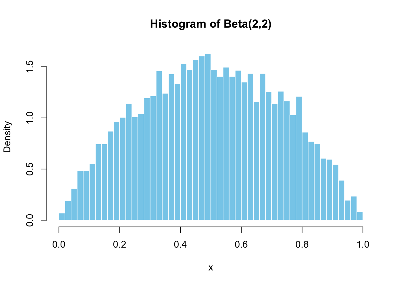
Start with a prior belief about \(p\), say we think it’s probably fair but not quite certain, we can assume \(p\sim Beta(2,2)\) where on average \(p=0.5\) but with some uncertainty. (Yes! In Bayesian, parameter is treated as a random variable with its own distribution.)

set.seed(123)
x <- rbeta(10000, shape1 = 2, shape2 = 2)
hist(x, breaks = 50, col = "skyblue", border = "white",
     main = "Histogram of Beta(2,2)",
     xlab = "x", freq = FALSE)

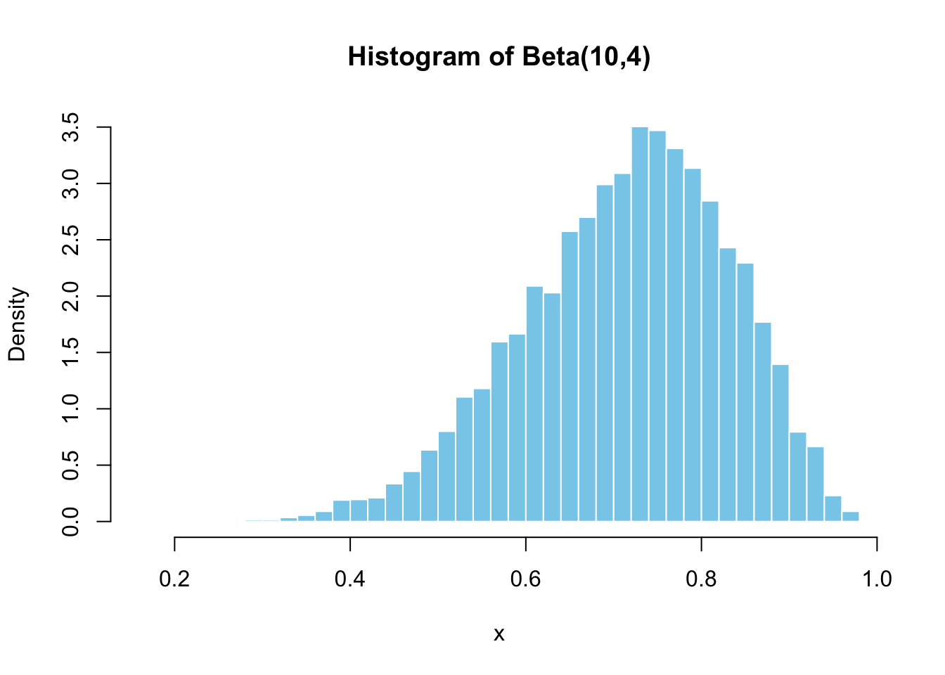
After seeing 8 heads, 2 tails, the posterior becomes (let’s ignore the math for now):

\[ p|\text{data} \sim \text{Beta}(2+8, 2+2) = \text{Beta}(10,4) \]

set.seed(123)
x <- rbeta(10000, shape1 = 10, shape2 = 4)
hist(x, breaks = 50, col = "skyblue", border = "white",
     main = "Histogram of Beta(10,4)",
     xlab = "x", freq = FALSE)

Since the data suggests that the actual \(p\) should be higher than 0.5, the updated distribution of \(p\) is skewed to the left. That is a direct probabilistic statement about the parameter, which frequentist methods can’t make. From this distribution, we can compute exactly that “there is a 95% probability that the coin’s bias \(p\) lies between 0.46 and 0.91”.

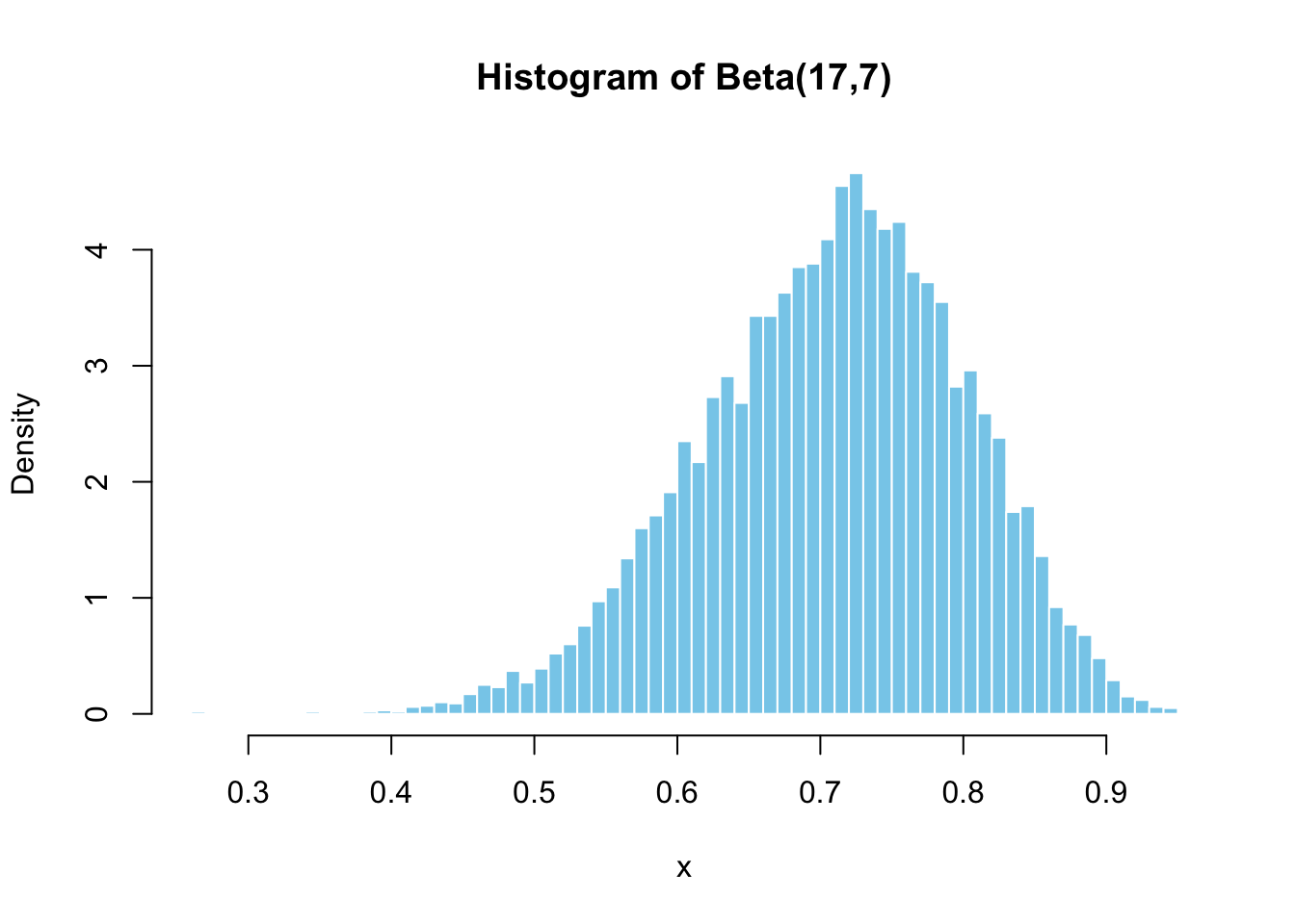
Now suppose another 10 experiments give us 7 heads and 3 tails, then we update the posterior again

\[ p|data \sim Beta(2+8+7, 2+2+3) = Beta(17, 7) \]

set.seed(123)
x <- rbeta(10000, shape1 = 17, shape2 = 7)
hist(x, breaks = 50, col = "skyblue", border = "white",
     main = "Histogram of Beta(17,7)",
     xlab = "x", freq = FALSE)

The interval estimate can now be interpreted as “there is a 95% probability that the coin’s bias \(p\) lies between 0.52 and 0.87”. In theory, this posterior distribution can be updated each time new experimental data are collected, allowing beliefs about \(p\) to evolve sequentially.

Aspect	Frequentist	Bayesian
What is probability?	Long-run frequency of outcomes	Degree of belief about uncertainty
Parameters	Fixed but unknown	Random variables with distributions
Prior knowledge	Ignored (data-only inference)	Explicitly included via the prior
Output	Point estimates, p-values, confidence intervals	Posterior distributions, credible intervals
Interpretation	What would I see if I repeated this experiment many times?	Given what I’ve seen, what should I believe now?
Change Point Detection	Fit all possible segmentations, pick the one that minimizes RSS + penalty.	Update the posterior probability of change for each day but no deterministic results.

Bayesian Inference in Change Point Detection

In the context of change-point detection, the Bayesian idea is the same:

• Define a prior belief about how often changes occur.

• Use data to update the probability that a change happened at time \(t\).

So the algorithm updates

\[ P(\text{Change point at time } t | \text{data up to } t) \]

Each time a new point arrives, this probability gets updated for a dynamic system.

The Run Length

The key quantity we tracks is the run length \(r_t\)

• \(r_t=0\) : a new change just occurred at time \(t\);
• \(r_t = 5\): the current regime (no change period) has lasted for 5 observations.

At each time step, the algorithm maintains a probability distribution over all possible run lengths:

\[ P(r_t|x_{1:t}) \]

that means, “given all the data so far, what is the probability that the current run has lasted \(r_t\) points?”.

Recursive Algorithm

At time \(t\), we should have the distribution of the parameter up to time \(t-1\). When the next data point \(y_t\) arrives, we need to do the following steps: (please note these are conceptual steps for pedagogy, NOT the authentic derivation)

1. Predictive probability for new observation, compute the predictive likelihood of the new data point

\[ p(x_t | x_{1:t-1}, r_{t-1}) \] This depends on your chosen distribution. For example, the assumed distribution could be Normal

2. Compute the growth probability. Here, we can assume a constant hazard where

\[ P(r_t = r_{t-1} + 1|r_{t-1})=1-h, \text{ if no change point occurs} \]

and the change point probability

\[ P(r_t = 0|r_{t-1})=h, \text{ if a change point occurs} \]

To “grow”, we need \(r_t=r_{t-1}+1\) , then the joint distribution of \(r_t\) and \(x_{1:t}\) is

\[ P( x_{1:t}, r_t=r_{t-1}+1) = P(x_{1:t} \ \ | \ \ r_t) \ \ P(r_t) = (1-h) \ \ P(x_{1:t}\ \ | \ \ r_{t-1}) \]

\[ =(1-h) \ \ P(x_t \ | \ x_{1:t-1}, \ r_{t-1}) \ \ P(x_{1:t-1}, \ \ r_{t-1}) \]

3. Compute the changepoint probability. To “stop”, we need \(r_t=0\) with a constant hazard. Then the value of \(r_{t-1}\) can be anywhere between 0 to \(t-1\) . So we will need to sum over all possible \(r_{t-1}\) .

The growth probability and changepoint probability provides all possible situations for \(r_t\) .

\[ P(x_{1:t}, r_t) = P(x_{1:t}, \ \ r_t = 0) + P(x_{1:t} \ , \ r_{t} = r_{t-1} + 1) \]

4. To get the posterior, (conditional on the data, what is the probability that a change occurs at time \(t\)), we normalize over all possible run lengths such that the probabilities sum up to 1.

\[ P(r_t| x_{1:t}) = \frac{P(x_{1:t}\ , r_t)}{P(x_{1:t})}=\frac{P(x_{1:t}, \ r_t)}{\sum_{r_t = 0}^{t} P(x_{1:t} \ , \ r_t)} \]

5. Repeat steps 1-4 when moving to the next time step \(t+1\).

For more detailed derivation, check the reflection blog “Bayesian Online Changepoint Detection” written by Gregory Gundersen.

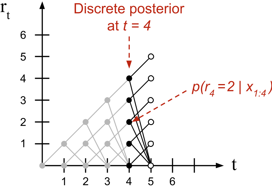
We can visualize the message-passing algorithm as living on a trellis . At each time point, mass is either passed “upward” such that the run-length is incremented or “downward” where it is truncated to zero. At each time point \(t\), there are \(t+1\) possible values of \(r_t\) . The “message passing” diagram shows the relationship between all possible paths. For example, the probability of \(P(r_4 = 2|x_{1:4})\) is associated with the node indexed by \(t=4\) and \(r_t=2\) .

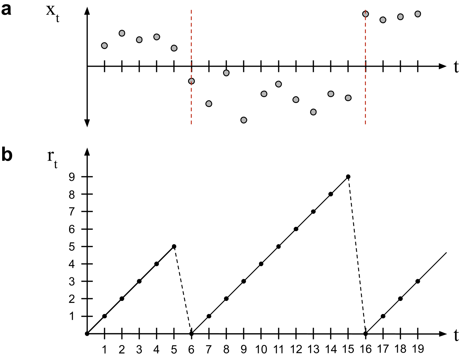
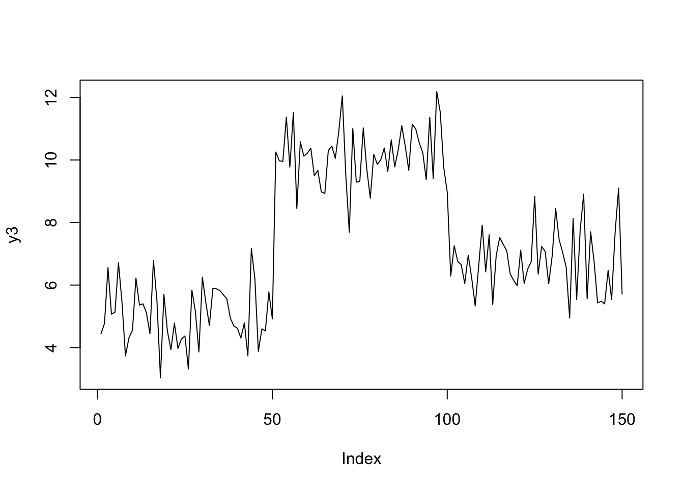
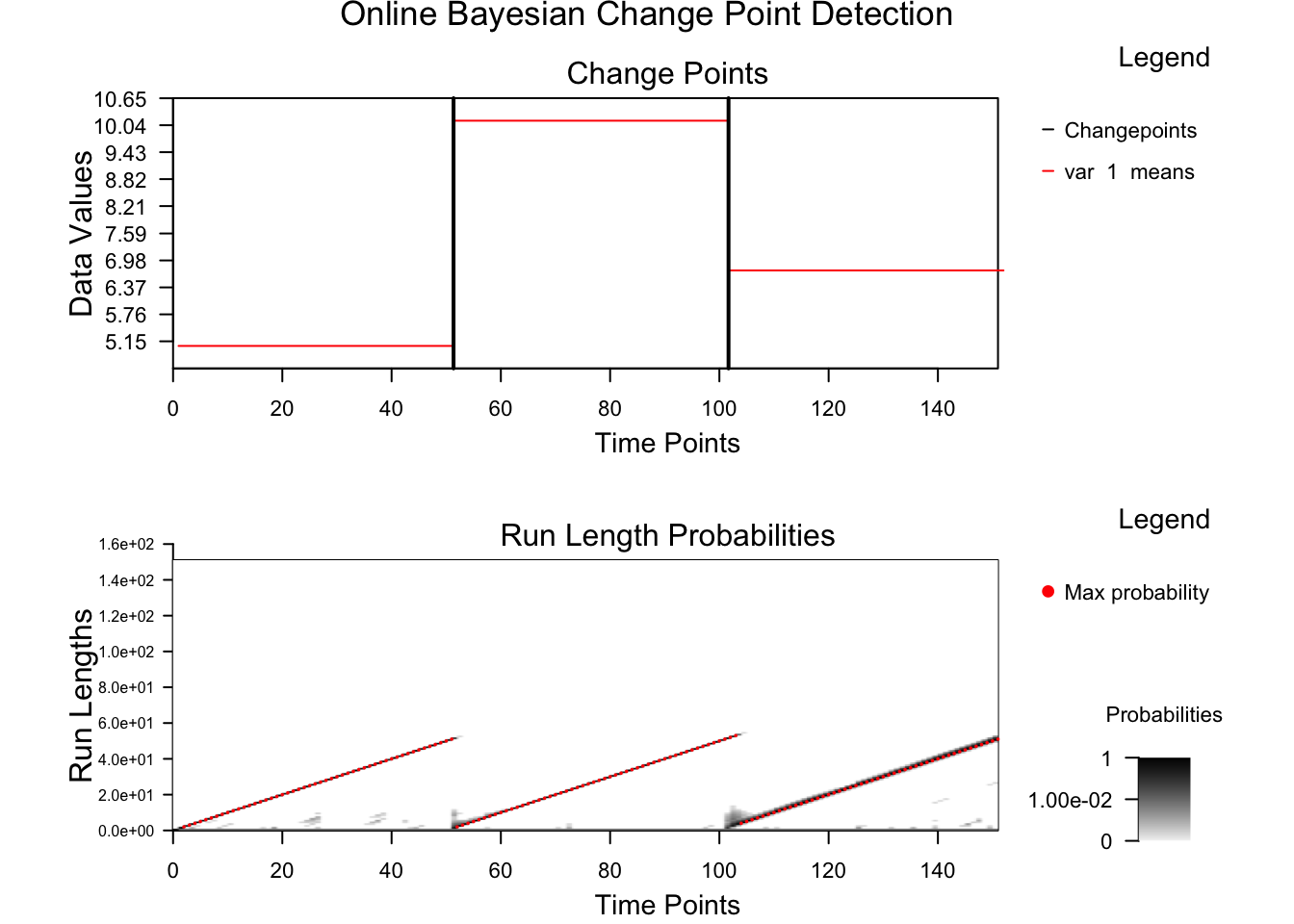
This conceptual diagram shows synthetic data divided into three segments by two change points. The corresponding run length \(r_t\) evolves over time \(t\), it increases within each segment and resets to zero whenever a change point occurs.

library("ocp")
set.seed(123)
y3 <- c(rnorm(50, 5, 1), rnorm(50, 10, 1), rnorm(50, 7, 1))
plot(y3, type = 'l')

# running the basic function with all the default settings
ocp_result <- onlineCPD(y3, getR=TRUE)
summary(ocp_result)

[1] "  An oCPD object:"
[1] "R vectors not truncated."
[1] "1 -variate data."
[1] "Attributes returned:"
 [1] "R"                 "prevR"             "prevRprod"        
 [4] "prevRsum"          "prevDataPt"        "time"             
 [7] "ocpd_settings"     "threshcps"         "max"              
[10] "update_paramsT"    "update_params0"    "init_params"      
[13] "logprobmaxes"      "logprobcps"        "currmu"           
[16] "changepoint_lists"
[1] "Changepoints:"
[[1]]
[1]   1  51 101

plot(ocp_result, main = "Online Bayesian Change Point Detection")

Interpretation

• Within-segment Posterior Mean

  • Posterior means intervals tell you where the levels differ across segment.

• Run-length Probabilities:

  -A distribution over “how many points since the last change” at each time \(t\).

  • A spike at \(r_t=0\) means that a new segment just started.
  • High mass at large \(r_t\) means the current segment has persisted for a while.
  • A vertical bright band near \(r=0\) means “detected change”.

• Change point probability (the grey scale shade):

  • Values near 1 means “strong evidence of a change at \(t\)”, near 0 means “no change”
  • Set a threshold (e.g. 0.8? 0.7?) to flag a change point in real time.

• Max probability: most possible segmentation.

  • A single best guess of where the breaks occur.
  • Max probability pass is convenient, but hides uncertainty. Pair it with the run-length plot.

Other interpretation tips:

• A sharp jump in change point probability followed by a short run length indicates fast detection.

• A slow rise in change point probability with moderate run length shows gradual or weak change, may expect longer detection delay.

• If multiple nearby times show nontrivial change probability, the exact change point is uncertain. Typically report a change window.

• If the run-length posterior keeps resetting, either the data truly change too often, or the model is too sensitive, e.g. hazard function is too high, allowed variance is too small.

• Sanity check: plot raw data with shaded change interval and segment posterior means: does the visual story match the model?

• Sensitivity check: refit the model with different hazard \(h\) to see if breakpoints are robust.

• Cross validation: test the algorithm on known “stable” data, or known “labeled” date. If change point probabilities rise high on stable data, you are overfitting. If no known change point is detected, you are underfitting.