Code
x <- rbeta(10000, 1,1)
hist(x)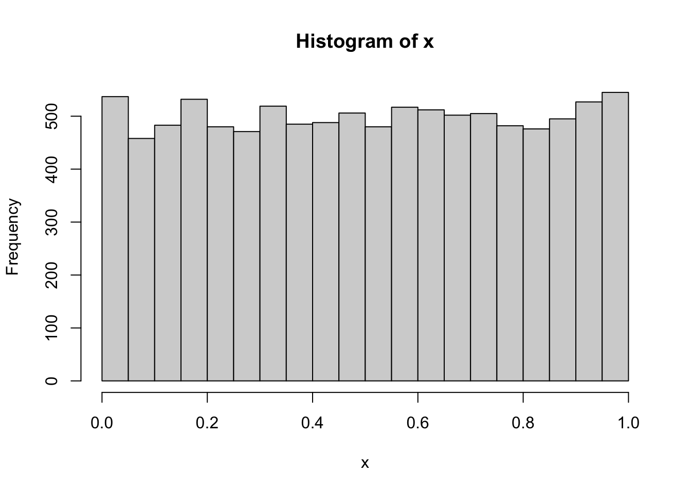
Sequential Fixed-width Confidence Interval
Sequential Probability Ratio Test
Sequential Shewhart chart, CUSUM chart and EWMA chart
Sequential Adaptive Design with Alpha Spending Function
Swinging Door Algorithm
Bayesian Online Change Point Detection
When we set \(\alpha=0.5\) as the significance level, we’re aiming to cap the probability of a Type I error (a false positive) at 5% under the test’s assumptions. But what’s the actual false positive rate in practice? We can estimate it empirically with a simulation.
Imagine an A/B test where the landing page shows one of two logos (A or B). The goal is to see which logo leads to more conversions. Below are examples of A and B:

Recall: a Type I error occurs when we reject the null hypothesis even though it is true. In most applications the null encodes a “no effect” claim (no difference, no disease, no changepoint, same distribution, etc.). Hence, under a true null, the Type I error probability is the false positive rate.
For each visitor, there are two possible outcomes: click the logo or not click the logo. Let the underlying conversion probability be p. We model a single visitor’s behavior with a Bernoulli random variable. \[ X \sim \text{Bernoulli}(p), E(X)=p, V(X)=p(1-p) \]
where \(X=1\) denotes a click.
For a group of \(n\) independent visitors exposed to the same version, the total number of clicks is
\[ \sum_{i=1}^nX_i \sim \text{Bin}(n,p), E(X)=np, V(X)=np(1-p) \] In an A/B test, we fit this model separately for each variant, using \(p_A\) and \(p_B\) and their binomials: Bin(\(n_A,p_A\)) and Bin(\(n_B, p_B\)).
Assumptions: visitors are independent and identically distributed within each variant, and each visitor has a single eligible exposure. If these are violated (e.g., repeat exposures, strong heterogeneity), you may need stratification or hierarchical models.
Among the \(n_A\) visitors randomly assigned to design A, \(x_A\) clicked the button; in group B, \(x_B\) clicked out of \(n_B\). The conversion rates are estimated by
\[ \hat{p}_A = \frac{x_A}{n_A}, \hat{p}_B = \frac{x_B}{n_B} \]
where \[ V(\hat{p}_A)=\frac{p_A(1-p_A)}{n_A}, V(\hat{p}_B) = \frac{p_B(1-p_B)}{n_B} \]
To evaluate whether A outperforms B,
\[ H_0: p_A -p_B = 0 , H_a: p_A - p_B >0 \] Under \(H_0\), let’s assume
\[ p_A = p_B = p \] Then the overall conversion probability can be estimated using a pooled estimator: \[ \hat{p}=\frac{x_A+x_B}{n_A+n_B} \] Plug it in the previous variance of the estimator, we have \[ \hat{V}({p}_A)=\frac{\hat{p}(1-\hat{p})}{n_A}, \hat{V}(p_B) = \frac{\hat{p}(1-\hat{p})}{n_B} \]
By central limit theorem, the test statistic is \[ Z_{Test}=\frac{\hat{p}_A-\hat{p}_B}{\sqrt{\hat{p}(1-\hat{p})(\frac{1}{n_A}+\frac{1}{n_B})}} \] The p value can be calculated as \[ \text{P Value} = P(Z\geq Z_{Test}), Z\sim N(0,1) \]
To “mimic” the false positive rate, we simulate data under the null hypothesis—that is, we assume the two versions have the same conversion probability. For example, let \(p_A = p_B = 0.3\), and suppose each version receives \(n_A = n_B=100\) visitors(though in practice the sample sizes need not be equal).
In each iteration,
Generate 2 random count \[ x_A \sim Bin(100, 0.3), x_B \sim Bin(100, 0.3) \]
Compute the test statistic \(Z_{Test}\) using \(x_A, x_B, n_A, n_B\).
Compute and record the corresponding p-value.
Repeat this procedure for 100000 iteration, the empirical distribution of p-values should show that
about 1% of the p values are below 0.01,
about 5% of the p values are below 0.05,
about 10% of the p values are below 0.1,
and in general, about a% of the p values are below a%.
In other words, when the null hypothesis is true, the p value follows a uniform[0,1] distribution. The practical significance level (false positive rate) should be very close to the pre-defined \(\alpha\).
When conducting a sequential (online) A/B test with multiple interim looks (e.g., reviewing the results after 10, 20, 30, … visitors), the actual false positive rate may be much larger than the nominal significance level \(\alpha\). Without appropriate adjustments, such as alpha-spending, group-sequential boundaries, or anytime-valid p-values, repeated peeking can inflate Type I error well beyond the intended level.
“Peeking” in A/B testing means checking significance before the preplanned final sample size and stopping early when a p-value looks “significant.” To better understand how “peeking” and repeated looks inflate the Type I error rate, let’s conduct another simulation study.
In this simulation, instead of simulate one random count from Bin(100, 0.3), we simulate the count for each interim look (10,20, 30,…,100). In each iteration:
For looks \(l=1,2,..,10\), independently draw \[ x_{A,l} \sim Bin(10,0.3), x_{B,l} \sim Bin(10,0.3) \]
At each look \(l\), compute \(Z_{Test,l}\) and it’s p value from \(x_{A,l}\), \(x_{B,l}\), \(n_{A,l}=n_{B,l}=10\).
If any p-value < 0.05, stop and record the first significant p value; otherwise record the p value at the last look when \(l=10\).
Repeat this procedure for 100000 iteration, and estimate the empirical type I error rate:
What proportion of the p values fall below 0.1?
What proportion of the p values fall below 0.05?
What proportion of the p values fall below 0.01?
and in general, what proportion of the p values fall below a%?
When conducting group sequential A/B test with multiple interim looks, each extra look is another chance to get a false positive (i.e. to see a small p-value just by chance).
If you stop at the first significant look, the observed effect size at that stop tends to be overestimated (you stopped on a high fluctuation). Reported CIs at that look have undercoverage unless adjusted for the stopping rule.
Early tiny p’s are overrepresented and late non-significant p’s are censored. Naively pooling such p’s gives misleading summaries. The distribution is no longer uniform.
For this type of test, we will need to control the familywise error(FWER): the probability of making at least one type I error (false positive) across a set (“family”) of hypotheses tested together. In general, if you test \(L\) times at level \(\alpha\) and the looks are independent, the probability of getting any false positive(reject at least one true \(H_0\)) is:
\[ FWER=P(\text{any false positive}) = 1-(1-\alpha)^L \] Even with correlated looks (typical, due to cumulative data), the error still rises well above 0.05.
When we think about multiple comparisons, methods like Tukey’s HSD or Bonferroni often come to mind. But are they actually useful in a peeking scenario?
What is Tukey’s HSD?
Tukey’s HSD is a post-hoc multiple comparison procedure usually after one-way ANOVA to find which pairs of the group means differ, while controlling familywise error(FWER) at \(\alpha\). It uses a studentized range distribution \(q\) to set a common critical difference. A pair \((i,j)\) is significant if \(|\bar{y}_i - \bar{y}_j|>q \sqrt{\frac{MSE}{n}}\).
Tukey’s HSD doesn’t fix peeking, because peeking is sequential monitoring over time, not a set of simultaneous pairwise mean comparisons.
What is Bonferroni correction?
Short answer: test each look at \(\alpha/L\) level(e.g. 10 looks, so per look \(\alpha=0.005\)). Bonferroni doesn’t require independence and controls FWER to be lower than \(\alpha\) even though looks are correlated.
However, in online-monitoring, you can’t pre-fix \(L\)(early termination, unplanned peeking, etc.), and Bonferroni is conservative, reducing the statistical power (true positive rate).
We need a method whose p-values stay valid no matter when we stop, even with continuous monitoring and data-dependent stopping. A popular choice is the mixture SPRT (mSPRT).
The classic SPRT compares a simple (point) \(H_0: \theta=\theta_0\) to a simple (point) \(H_a:\theta=\theta_1\). mSPRT replaces the simple alternative by a mixture over alternatives and compute a likelihood ratio averaged over all plausible effects(prior). The full theory is beyond our course scope, so here’s the intuition:
Pick a small manue of plausible effects (the “mixture”) rather than a single fixed value for the alternative.
Update how well each effect explain the data via likelihood.
Combine them into one running evidence number: the likelihood ratio(\(\Lambda_t\)).
Stop and declare a win the first time \(\Lambda \geq 1/\alpha\).
A convenient always-valid p value is
\[ p_t = min\{1, \frac{1}{LR_t}\} \]
When computing the likelihood under \(H_0\) and \(H_a\), we bring in the idea of “prior”. For example, in the previous AB test, put a Beta prior on \(p\sim \text{Beta}(1,1)\). As a refresher, here is the what a Beta(1,1) distribution looks like. Yes that’s exactly Uniform(0,1).
x <- rbeta(10000, 1,1)
hist(x)
It’s often called a “noninformative” prior or a “flat” prior. Because it does not push the posterior in any particular direction, it is commonly used when:
you have no prior belief about the conversion rate
you want the posterior to be dominated by the data
you want a neutral baseline for A/B tests.
Most AB testing platform like Google often start with Beta(1,1) prior for conversion rates, click-through rates, or success probabilities. It lets us compare posteriors with minimal subjective influence.
The posterior distribution is still a Beta distribution(see results in Bayesian Online Change Point Detection notes) as Beta(1+“success”, 1+“failure”).
Under \(H_0\), we put \(p_A=p_B=p\sim \text{Beta}(1,1)\). Then the posterior likelihood is
\[ L_0 = \frac{\text{Beta}(1+x_A+x_B, 1+n_A-x_A+n_B-x_B)}{\text{Beta}(1,1)} \]
Under \(H_1\), we put \(p_A\sim \text{Beta}(1,1)\), \(p_B\sim \text{Beta}(1,1)\). Then the posterior likelihood is \[ L_1=\frac{\text{Beta}(1+x_A, 1+n_A-x_A)}{\text{Beta}(1,1)} \frac{\text{Beta}(1+x_B,1+n_B-x_B)}{\text{Beta}(1,1)} \] Then the mixture likelihood ratio is \[ \Lambda_t = \frac{L_1}{L_0} \] Stop and reject the first time \[ \Lambda_t>\frac{1}{\alpha} \]
Then the always valid p-value is \[ p=\text{min}\{1,\frac{1}{\Lambda_t}\} \] This method guarantees at each time \(t\), \(P(\text{p value}\leq \alpha)\leq \alpha\). So you can peek anytime and stop when evidence crosses a boundary, without inflating Type I error.